Analysis of the phase portrait of a nonlinear system
A nonlinear automatic control system is a system that contains at least one link, which is described by a nonlinear dependence. The internal model of a nonlinear system is composed of equations
|
|
(1) |
where ![]() — state vector;
— state vector; ![]() — output vector and control vector;
— output vector and control vector; ![]() — nonlinear vector differential equations[1].
— nonlinear vector differential equations[1].
For the analysis of nonlinear systems use the concept of phase space ![]() .
.
In a real control system, the coordinates of the system state ![]() at each instant have completely definite values, this corresponds to the well-defined position of the image point M in the state space. Over time, values of
at each instant have completely definite values, this corresponds to the well-defined position of the image point M in the state space. Over time, values of ![]() changes, which corresponds to the displacement of the point M along an oriented curve, called the phase trajectory in the phase space X (Fig. 1). The set of phase trajectories is called the phase portrait of the system. To determine the phase portrait of the system, it is necessary to find solutions of the differential equations that make up the system model. The phase portrait of a nonlinear system, in contrast to the phase portrait of a linear system, is generally heterogeneous. A nonlinear system can have a countable or continuous number of singular points[2].
changes, which corresponds to the displacement of the point M along an oriented curve, called the phase trajectory in the phase space X (Fig. 1). The set of phase trajectories is called the phase portrait of the system. To determine the phase portrait of the system, it is necessary to find solutions of the differential equations that make up the system model. The phase portrait of a nonlinear system, in contrast to the phase portrait of a linear system, is generally heterogeneous. A nonlinear system can have a countable or continuous number of singular points[2].
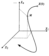
Fig. 1. Phase trajectory of the system movement
Stabilization of nonlinear regulation systems
When analyzing linear control systems, sometimes, as a rough estimate of their quality, the maximum value of the output to the input ratio of the Mm system is considered when the signal frequency at the input changes from 0 to µ. It is considered that the system, to a first approximation is satisfactory, if Mm <1.3… A similar quality assessment method can be used in the study of a nonlinear system. In this case, the results should be considered, of course, as the first rough approximation[3].
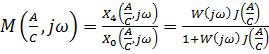
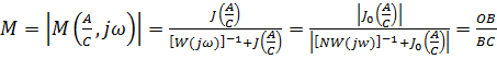
Consider a nonlinear tracking system whose structural diagram is shown in Fig. 2. If the input quantity x0 changes according to a harmonic law, and in a nonlinear system there arise oscillations whose first harmonic has a frequency of the input quantity, then we can write the following relation:
|
|
(2) |
where
W(jw)=W1(jw) W2(jw);
A- the amplitude of the quantity x2 at the input of the nonlinear element.
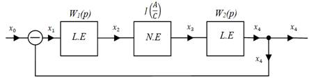
Fig. 2. Structural diagram of a tracking system
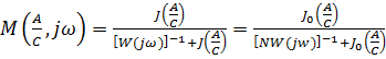
Equation (2) can be represented as
![]() (3)
(3)
or
|
|
(4) |
In the first case, to graphically determine M(jw), it is necessary to construct the
amplitude-phase frequency characteristic — NW(jw), and the equivalent characteristic ![]() in the second case —
in the second case —![]() and
and ![]() , respectively.
, respectively.
We will use the second, in this case, more convenient, trick. The amplitude-phase frequency characteristic and characteristic —![]() are shown in Fig. 3. We determine the value of
are shown in Fig. 3. We determine the value of ![]() for a given value of the amplitude
for a given value of the amplitude ![]() and frequency w. The amplitude
and frequency w. The amplitude ![]() determines the point B, the frequency w determines the point C (see Fig. 3). According to equality (4) and Fig. 3 we have
determines the point B, the frequency w determines the point C (see Fig. 3). According to equality (4) and Fig. 3 we have
 (5)
(5)
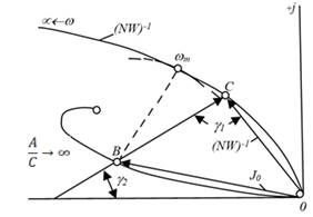
Fig.3.Amplitude-phase frequency characteristic and equivalent amplitude-phase characteristic of a nonlinear system
For a given value ![]() , the segment OB remains constant, and thus the value M will change with frequency fluctuations w due to changes in the segment BC . The value of M will be maximum with a minimum value of BC:
, the segment OB remains constant, and thus the value M will change with frequency fluctuations w due to changes in the segment BC . The value of M will be maximum with a minimum value of BC:
|
|
(6) |
The value of BCmin is defined as the minimum radius of a circle touching the amplitude-phase frequency response and having a center at point B. The frequency at the point of contact (Fig. 3), corresponding to the maximum of M, is denote wm. With this construction, for each value of ![]() , Mm and wm can be determined. In Fig. 4
, Mm and wm can be determined. In Fig. 4
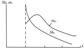
Fig.4. Graph of the dependence of Mm and wm on ![]()
shows the form of the curves Mm![]() and wm
and wm![]() for a particular case. For large quantity of
for a particular case. For large quantity of ![]() , the value of Mm is less, and therefore, we can assume that the development of large perturbations occurs with smaller fluctuations than the processing of small ones. Satisfactory results are obtained if the highest value of Mm is less than 2 and for large values of
, the value of Mm is less, and therefore, we can assume that the development of large perturbations occurs with smaller fluctuations than the processing of small ones. Satisfactory results are obtained if the highest value of Mm is less than 2 and for large values of ![]() does not exceed 1.3[4].
does not exceed 1.3[4].
In cases where the quality of the regulatory process is unsatisfactory, by introducing corrective circuits, we deform the amplitude-phase frequency response, which will significantly improve the nature of the transition process.In the example of a relay tracking system, it was possible to obtain relatively satisfactory results by increasing the deadband (decreasing the value of N), and significantly better results were obtained using a correction loop of resistance and capacitance. The transition process in the second case is more satisfactory, and the deadband was reduced by about 8 times[5].
Consider a system of the following form (Fig. 5):
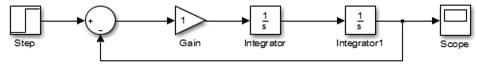
Fig. 5. Block diagram of a closed-loop control system
The analysis of such a system by methods of the automatic control theory shows that undamped oscillations (conservative system) will exist in it.
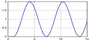
Fig. 6. Schedule of the transition process
The phase portrait of the system is shown in Fig.7.
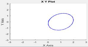
Fig. 7. The phase portrait of the system
The phase portrait looks like an ellipse. By changing the gain k, can change the shape of this ellipse by stretching it along one axis or another. Assume that the phase portrait of the system shown in fig. 7 corresponds to the gain k1=2, then with a different gain k2=0.5 , the type of phase portrait can be like this (Fig. 8):
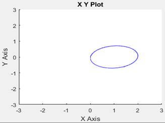
Fig. 8. The phase portrait of the system
Now imagine that at first the system moves along the phase trajectory of fig. 7 (gain k1), but when the x1 axis crosses the image point, the gain changes to k2. Then, at the intersection of the x2 axis, it changes again to k1, and at the next intersection of x1, it again to k2. In other words, the change of coefficients occurs when the sign of the product ![]() changes. Then the phase portrait of the system will be as shown in Fig. 9.
changes. Then the phase portrait of the system will be as shown in Fig. 9.
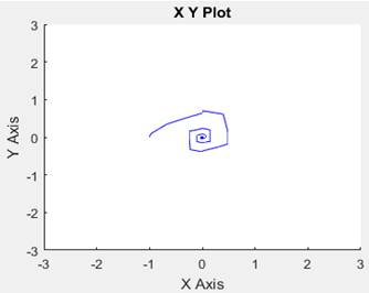
Fig. 9. The phase portrait of the system
That is, a change in the gain when changing the sign ![]() allowed us to turn a system with undamped oscillations into a stable system.
allowed us to turn a system with undamped oscillations into a stable system.
How can organize a change the gain? For example, this: have two control programs, one for the case k1, the other for the case k2. When the sign ![]() changes, the special device switches to the corresponding program (fig. 10).
changes, the special device switches to the corresponding program (fig. 10).
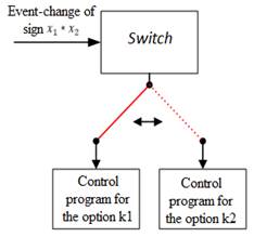
Fig. 10. Change of gain
The role of such a switch is played by the operating system, which launches the corresponding control program when the event of changing the sign of the product ![]() occurs.
occurs.
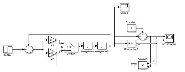 Fig. 11. Block diagram of a mathematical model of the system
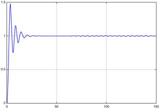
Fig.12. Schedule of the transition process
Conclusion
The phase trajectory in the phase plane gives a geometric idea of the system under study dynamics . The phase plane is a two-dimensional coordinate plane with two phase coordinates, an adjustable quantity x1 and its first derivative x2.
By changing the initial conditions or the initial state, we change the phase trajectory so as to achieve stability of the system. Switching is carried out in the control program of the controller.
References
1. Лазута И.В., Щербаков В.С.Теория автоматического управления. Нелинейные системы. Омск: Учебное пособие,2017.-161 с.
2. Ким Д.П. Сборник задач по теории автоматического управления. Многомерные, нелинейные, оптимальные и адаптивные системы. М.: Физматлит,2008.-328 с.
3. Смирнов Н.В.,Смирнова Т.Е.,Тамасян Г.Ш. Стабилизация программных движений при полной и неполной обратной связи: Учебное пособие.– 3-е изд.,стер.– СПб.:Издательство «Лань», 2017.–128 с.
4. Коновалов Б.И., Лебедев Ю.М. Теория автоматического управления: Учебное пособие.–4-е изд.,стер.–СПб.: Издательство «Лань», 2016.– 224 с.
5. Кудинов Ю.И., Пащенко Ф.Ф. Теория автоматического управления (с использованием MATLAB–SIMULINK): Учебное пособие.– 3-е изд.,стер.– СПб.:Издательство «Лань», 2019.–312 с.