Introduction
Spain’s capitalist mixed economy is the 14th largest worldwide and the 5th largest in the European Union, as well as the Eurozone’s 4th largest.
After the financial crisis of 2007-2008, the Spain economy plunged into recession, entering a cycle of negative macroeconomic performance. In 2012 a quarter of Spain’s workforce left unemployed and reversed the economic boom of the 2000s. In aggregated terms, the Spanish GDP contracted by almost 9% during the 2009–2013 period. In 2013-2014 Spain managed to reverse the record trade deficit, attaining a trade surplus after three decades of running a trade deficit. In 2015 GDP of Spain has fallen, that can be described as a crisis time for the world’s economy, same as in 2007-2008.
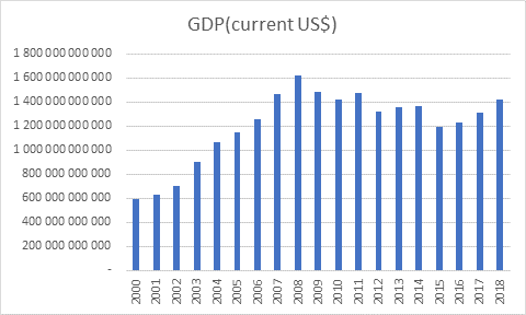
Table 1 GDP – Spain 2000-2018
Regression analysis
We performed a correlation analysis of the relationship between exogenous and endogenous indicators. At that rate, endogenous indicator is GDP. Considered period is since 2001 to 2018 year. Currently there is no actual data about 2019 year.
![]() – the endogenous parameter (the GDP), the aim of constructing this model.
– the endogenous parameter (the GDP), the aim of constructing this model.
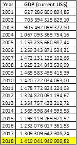
Figure 1 – The data for Y –the GDP in Spain
Let us consider the major factors (variables), which influence on GDP. There are four exogenous parameters in this model. The GPD is the first one, which are taken with the lag. The lag is equal to one year.
![]() – the lagged GDP.
– the lagged GDP.
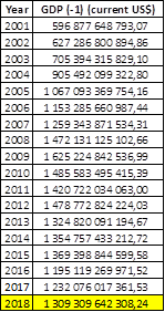
Figure 2 – The data for X1 – lagged GDP
The second parameter for our model is the general government final consumption expenditure.
![]() – the general government final consumption expenditure.
– the general government final consumption expenditure.
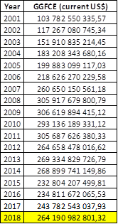
Figure 3 – The data for X2 – general government final consumption expenditure
The third parameter is the general government final consumption expenditure, that taken with lag. Lag is equal to one year.
![]() – the lagged general government final consumption expenditure.
– the lagged general government final consumption expenditure.
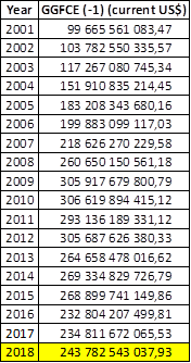
Figure 4 – The data for X3 calculation the lagged general government final consumption expenditure
The fourth parameter for our model is the final consumption expenditure.
![]() – the final consumption expenditure.
– the final consumption expenditure.
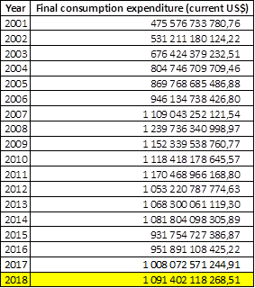
Figure 5 – The data for X4– final consumption expenditure
Creating the linear equation, by using the linear regression function in Excel, which calculate coefficient for each exogenous parameter. It that case, it is possible to estimate the relevance of the model.
Results
Our estimated model is presented below.
![]()
Coefficient of determination (R2adj) equals 0,999219014325001. This means that around 99.9% of the changes of the dependent variable are explained by the changes in the independent variables by the linear regression model.
F-test checks non-randomness of R2 and equality of specification of a linear regression model. From calculations it was received, that Fcrit=2,964 and F=5118,73286662037. This means that the coefficient of determination is non-random and quality of specifications on the estimated model is high.
The next step is completing T-test, comparing T-statistic with P-value. As we can see from the table 2, in absolute value, the T-statistic is higher than the P-value for all coefficients and we may conclude that our coefficients of linear regression are significant.
Table 2 – The data for T-test
|
T-statistic |
P-value |
|
-0,871564562 |
0,400547566 |
|
5,380276425 |
0,000165281 |
|
-1,179851151 |
0,260920814 |
|
-7,152132962 |
1,16082E-05 |
|
17,15821513 |
8,28035E-10 |
Next step is check by three Gauss-Markov conditions. The first condition of Gauss-Markov theorem is that average mean of residuals is equal to zero. In order to check that, the average mean of residuals should be calculated. As it can be seen from the residual table, the average mean of residuals is nearly equal to zero, henсe the first condition of Gauss-Markov theorem is satisfied. This means, that coefficients of the model are unbiased.
The Goldfeld-Quandt test can be used to check the second Gauss-Markov condition. This test checks the homoscedasticity in regression analyses. As it can be seen from the table 3, Fcrit is higher than GQ and 1/GQ.
Table 3 – The Goldfeld-Quandt test calculation
|
GQ |
6,469121916 |
|
1/GQ |
0,154580484 |
|
FcritGQ |
99,16620137 |
The Durbin-Watson test can be used to check the third Gauss-Markov condition. As it can be seen from the results of the test, Durbin-Watson value lies in the yellow zone between dl and du. This means that there is no information about autocorrelation.
Adequacy of the model is checked throughout the construction of the confidence interval. If the real value lies between Y^– and Y^+, then model is adequate. As it can be seen from the table 3, the real value stay between Y^– and Y^+, that’s why the model is adequate.
Table 4 – The Goldfeld-Quandt test calculation
|
Y^2018= |
1 420 914 283 528,75 |
|
Y^–2018= |
1 404 192 968 784,24 |
|
Y^+2018= |
1 437 635 598 273,25 |
|
Y2018= |
1 419 041 949 909,82 |
Finally, the average approximation variance is equal 0,132%, so this model is relevance for using.
BIBLIOGRAPHY
1. Трегуб И.В. Прогнозирование экономических показателей на рынке дополнительных услуг сотовой связи. Финансовая акад. при Правительстве Российской Федерации, Каф. Мат. моделирование экономических процессов. Москва, 2009.
2. Трегуб И.В. Математические модели динамики экономических систем: монография – Москва: РУСАЙНС, 2018. – 164 с.
3. Трегуб И.В. Эконометрические исследования. Практические примеры. Econometric studies. Practical examples. – Москва: Лань, 2017. 164 с.
4. Tregub I.V. Econometrics. Model of real system. М.: 2016, 164 p.
5. Трегуб И.В. Эконометрика на английском языке Учебное пособие. М.: 2017.3.
6. Financial data. https://data.worldbank.org/ [Accessed 24 February 2020].
7. Data and statistic https://countryeconomy.com/ [Accessed 28 February 2020]