Due to the fact that since 1990th the Russian Federation has been restructuring its economy to the market shape, some market attributes like currency exchange rate fluctuations have been appeared in Russian economy. If we consider the situation with the national currency exchange rate, the entire period of the Russian Federation might be subdivided on the two periods – before and after denomination 1998.
The first period (before denomination) is started since the creation of Russian Federation on the 25th of December 1991. At that period the Soviet banknotes have been circulated in the national economy. In 1993 these banknotes have been replaced on the new banknotes of Russian Federation within two weeks. The portrait of Vladimir Lenin and coat of arms of the USSR were removed and the towers of the Moscow Kremlin appeared on the new banknotes. These banknotes have been used till the denomination in 1998. The period from the creation of the Russian Federation till the 1998 was accompanied by hyperinflation and complete instability in the economy. As the result, the money was totally devalued and the wages were measured in million rubles to provide inconvenience for the economy as a whole. Due to the described above situation, it is difficult to do USD/RUB forecast, based on the economic parameters like inflation, interest rate in 1991-1997.
The second period (after the denomination up to the present time) may be considered as more stable than the first one. The hyperinflation has been disappeared and the Central Bank’s interest rate has begun to be measured in single-digits or double digits. However, the macroeconomic situation remained unstable. The level of inflation was 84,44%, 36,56%, 20,2%, 18,58% in 1998, 1999, 2000 and 2001 respectively. The interest rate fluctuated between 25% – 72,5% at the same period.
The final variant of the researched time framework was established on the 2008 for the modern variables and 2006 for the lagged variables till the end of 2018. It allows us to analyze independent factors before the crisis 2008 and their effect on the exchange rate.
To prepare econometric model for USD/RUB forecasts, it is necessary to identify the exogenous parameters. To be honest, there are a lot of economic events effect on the currency exchange rate. Some of them cannot be measured and included in the model such as statements of politicians, climate factors and so on.
However, the majority of unmeasured factors effect on the exchange rate temporarily to cause unexpected fluctuations on the foreign exchange market. Practically, the long-term dynamic and long-term forecasts do not involve these factors and based on the characteristics of the national economies. In our situation, the national economies are presented by Russian Federation and United States of America.
Let us consider the major factors (variables), which influence on the USD/RUB exchange rate.
The first parameter is inflation and it is better to compare the inflation value for both countries. Actually, if the level of inflation in one country is higher than in the second country, it will affect on the currency exchange rate. All things being equal, the currency of the first country will drop in relation with the currency of the second country.
There are two opposite views concerning the correlation and effects between inflation and exchange rate. The first one assumes that the national currency devaluation makes the import goods more expensive and it causes the growth of inflation. The second one has been partially explained above that inflation arises from internal economic problems of the country. It may be excess of money supply, shrinking the national production etc. In other words, the inflation influences on the currency exchange rate. Both explanations are truth and both parameters affect on each other.
However, in our model we consider the inflation as the exogenous (independent) variable and the exchange rate as the endogenous (dependent) variable, because the Russian currency exchange regime till the October of 2014 was called as managed float (or dirty float). The Central Bank controlled the exchange rate in the determined corridor. If the exchange rate broke these frames, the Central Bank made market intervention. It sold or bought the foreign currency to adjust exchange rate into diapason. That is why we cannot consider the foreign exchange as the explanatory (independent) variable.
Nowadays, the currency exchange regime is the free float and the present exchange rate involves all effects from inflation and other economic factors. The model will include the historical effects of inflation.
The interest rate is the second factor. As we know, when the Central Bank raises its interest rate, it causes exchange rate growth of the national currency. However, it is temporarily factor. The financial markets are strictly bound to each other. Investors try to earn some profit from the differences in the Central Banks’ interest rates. It is called as carry trade operation.
The operation has three major steps:
· investor acquires national currency of the country, where the Central Bank’s interest rate is higher;
· he makes deposit in this currency and wait period for the interest accrual;
· the deposit plus received percent are converted to the initial currency to fix the profit.
The major risk of this operation is the acquired currency devaluation during the period of deposit. If we consider carry trade operation for Russian ruble, it was possible to receive good yield, especially when the Central Bank of Russian Federation managed the exchange rate. The interest rate of Central Bank of Russian Federation has been higher than the interest rate of FED during the all observed period. Nowadays, the carry trade operation is also available for the foreign investor. The majority of foreign investor buy Russian government bond. The Central Bank of Russian Federation publishes the statistical information about the share of non-residents holders of the Russian government bonds. According to the information, the share of non-resident investments grows constantly. On the 01.01.2012 the share was 3,7%, on the 01.02.2020 it was 34,1%. The share of non-residents has been increased in ten times approximately.
As the result, when the bond is expired and foreign investors receive initial investment plus coupons, they convert it to US Dollar and transmit it from Russia. Surely, it has a negative impact on the USD/RUB exchange rate.
The third exogenous parameter is strictly related to the Russian economy specification. This is the price of oil. Obviously, if the price of oil increases, the USD/RUB exchange rate falls down. If the price of oil decreases, the opposite tendency can be observed in the USD/RUB exchange rate dynamic.
The fourth parameter is USD/RUB exchange rate, which are taken with the lag. The lag is equal one quarter. Definitely, the current exchange rate depends on its previous result and it is necessary to include this explanatory parameter in our model.
The inflation and the interest rate are the lagged parameters, which will influence on the exchange rate in the future. The lagged moment is equal two years (8 quarters) for both parameters, that is quite enough to pass the effect.
Based on the inflation and on the interest rate, some coefficients will be calculated.
The inflation will be presented by the level of inflation in Russia divided on the level of inflation in USA. The data are collected on the quarterly basis. The illustrative example of the calculation is presented below:
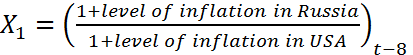 – it might be considered as the effective rate of devaluation. The calculation is related to the first item. After that, this variable includes the previous results. They will be multiplied one by one. In other words, X1 is the accumulated difference between inflation in two countries.
The same principle is applied for the interest rate (see below).
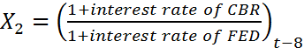 – the effective rate for carry trade operations. It is also accumulated parameter and calculation is related to the first item.
The price of oil is a modern variable. Practically, the changes in this parameter effects on the exchange rate immediately. The grade of oil in Russia is called Urals, in the USA – WTI. However, it is better to take another grade of oil for this parameter. The Brent is the most famous on the financial markets and its price fluctuation will be used in model. The average price of the Brent will be collected on the quarterly basis. The model relies on the linear regression.
![]() – the price of oil (Brent).
– the price of oil (Brent).
The last parameter (the lagged USD/RUB exchange rate) is based on the previous period data and complement the model.
![]() – the lagged USD/RUB exchange rate.
– the lagged USD/RUB exchange rate.
![]() – the endogenous parameter (the exchange rate), the aim of constructing this model.
– the endogenous parameter (the exchange rate), the aim of constructing this model.
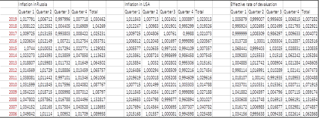
Figure 1 The data for further X1 calculation
The description of X1 parameter calculation is presented above, but the final step (does not show on the Figure 1) is the accumulating inflation effect through the periods to calculate the final value of X1.
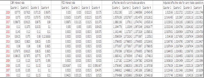
Figure 2 The data for further X2 calculation
The description of X2 parameter calculation is presented above, but it is necessary to comment the adjusted effective rate for carry trade operations.
Due to the fact that we collected data on the quarter basis. Each position of the interest rate effects on the quarter period. At the same time, the CBR and FED interest rates are measured on the annual basis. The interest rate was adjusted on the one-quarter degree (i^0,25). And the final step to calculate X2 is also calculating accumulated effect.
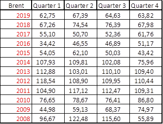
Figure 3 The average quarterly price of Brent (X3)
The collected data of the price of Brent (X3) are presented above.
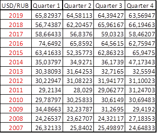
Figure 4 The USD/RUB exchange rate data
These data describe the endogenous parameter Y and lagged exogenous parameter X4.
By using the linear regression function in Excel, it is possible to create the linear equation, which calculate coefficient for each exogenous parameter. After that, we are able to do forecast, if the model satisfies specific requirements.
There are four principle of model specification.
The first principle of specification of economic model: specification of a model is a result of a translation of the economics laws into mathematical language. Actually, we have done it.
The second principle of specification of economic model: number of equations in the econometric model should be equal to the number of endogenous variables, included into a model. We have one endogenous variable (exchange rate) and one equation, which explains it.
The third principle of specification of economic model: each variable in the model should be dated, i.e. the moment of time when the variable is measured, should be clearly defined. Definitely, we know carefully the period of collected data and subdivided it on the lagged and modern variables. In other words, principle is fulfilled.
The fourth principle of specification of economic model: in the behavioral equation of the model should include disturbance term. Due to the fact, that we implement least square regression, it leads the appearance of disturbance term. The disturbance term plus forecast endogenous variable (calculated by the linear regression coefficients) will be resulted the actual value of endogenous parameter (USD/RUB exchange rate).
Our estimated model is presented below.
![]()
There are some rules and conditions allow us to use or not to use the constructed econometric model.
Firstly, we have to calculate the adjusted coefficient of determination. In our case, it is equal 0,95. It shows us that 95% of changes of dependent variable are explained by changes of independent variables by linear regression model.
The next rule is the completing T-test. We have to compare T-statistic with P-value.
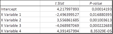
Figure 5 The data for T-test
In absolute value, the T-statistic is higher than the P-value for all coefficients and we may conclude that our coefficients of linear regression are significant.
In addition, we have three conditions of Gauss-Markov. If the model is appropriated for these conditions, it means that it was created properly.
The first condition is that the expected value of the disturbance term in any observation should be 0. In our case, the average distribution term tends to zero. In other words, the first condition is satisfied.
The second condition is that the population variance of the disturbance term should be constant for all observations. This situation is called as homoscedasticity. If the population variance of the disturbance term has a different value for all observation, it is called as heteroscedasticity. The model and its coefficients become ineffective as the explanation instrument of endogenous variable. For checking the second condition of Gauss-Markov, the Goldfeld-Quandt test is applied.
Table 1 The Goldfeld-Quandt test calculation
|
GQ = |
0,63569119 |
|
1/GQ = |
1,57309087 |
|
FcritGQ = |
2,40344707 |
The FcritGQ is higher for the both coefficients. It indicates that coefficients of the model are unbiased, consistent and accurate. The heteroscedasticity does not exist and the second Gauss-Markov condition is satisfied.
The third condition states that there should be no systematic association between the values of the disturbance term in any two observations. In other words, there is no autocorrelation between disturbance terms, no effects on each other.
If we have autocorrelation it means the value of disturbance terms of next observations depends on the previous disturbance terms. However, the disturbance term has to be occasional parameter. The third condition is checked by Durbin-Watson test.
The calculated DW coefficient is equal 1,86. This result is located between DU and 4-DU. It means there is no autocorrelation in residuals.
We have covered all necessary conditions and may forecast by implementing this model.
Let us make a two-year forecast for 2020-2021, because we have already collected data for two lagged parameters.
The price of oil is difficult to predict. Let us consider the pessimistic scenario, due to the fact, that OPEC arrangement of decreasing oil production tends to be expired. In the model forecast, we will use the average price for 2020 Q1 is equal 50$. The rest part of the year the average price is 40$ per barrel and 35$ per barrel in 2021.
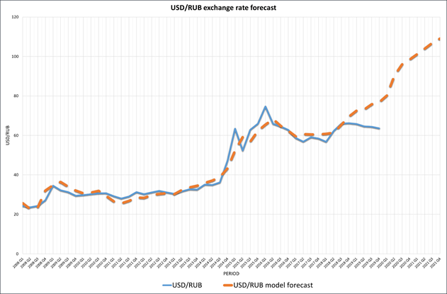
Figure 6 The graphical interpretation of the model forecast
Based on the model, which includes the accumulative effect of inflation and interest rate and low prices of oil (our prediction), we can announce the forecast on the 2020-2021 period. According to the model, in the middle of 2020 the USD/RUB will have breached the 80-level barrier. In the first quarter 2021, the USD/RUB trade pair will test the 100-level barrier and will have successfully breached it. In the end of 2021, the USD/RUB will be located on the 109 rub per 1$.
Definitely, it is rough model and we hope the real dynamic of USD/RUB will not be so dramatic. However, it is necessary to mention that current USD/RUB exchange rate (61 – 63 rubles per dollar) does not reflect macro-economic effects and the USD/RUB exchange rate will move up in the nearest future.
References
1. An, J., Dorofeev, M. Short-term foreign exchange forecasting: Decision making based on expert polls (2019) Investment Management and Financial Innovations, 16 (4), pp. 215-228.
2. Choi, M.S. The recent effects of exchange rate on international trade (2017) Prague Economic Papers, 26 (6), pp. 661-689.
3. Crespo Cuaresma, J., Fortin, I., Hlouskova, J. Exchange rate forecasting and the performance of currency portfolios (2018) Journal of Forecasting, 37 (5), pp. 519-540.
4. Fedoseeva, S. Under pressure: Dynamic pass-through of oil prices to the RUB/USD exchange rate (2018) International Economics, 156, pp. 117-126.
5. Kuzmenko, E., Smutka, L., Pankov, M., Efimova, N. The success of economic policies in Russia: Dependence on crude oil Vs. Export diversification (2017) Acta Universitatis Agriculturae et Silviculturae Mendelianae Brunensis, 65 (1), pp. 299-310.
6. Mele, M. A “time series” approach on the Chinese exchange rate regime (2010) Ekonomska Istrazivanja, 23 (3), pp. 1-11.
7. Plakandaras, V., Papadimitriou, T., Gogas, P., Diamantaras, K. Market sentiment and exchange rate directional forecasting (2015) Algorithmic Finance, 4 (1-2), pp. 69-79.
8. Tyll, L., Pernica, K., Arltová, M. The impact of economic sanctions on Russian economy and the RUB/USD exchange rate (2018) Journal of International Studies, 11 (1), pp. 21-33.
9. BCS Express broker website. https://bcs-express.ru [Accessed 3 March 2020].
10. CBR website. https://cbr.ru/ [Accessed 3 March 2020].
11. Financial data. https://www.investing.com [Accessed 3 March 2020].
12. Трегуб И.В. Математические модели динамики экономических систем: монография / И.В. Трегуб. – Москва: РУСАЙНС, 2018. – 164 с.
13. Трегуб И.В. Эконометрические исследования. Практические примеры. Econometric studies. Practical examples. – Москва: Лань, 2017. 164 с.
14. Tregub I.V. Econometrics. Model of real system. М.: 2016, 164 p.
15. Трегуб И.В. Эконометрика на английском языке Учебное пособие. М.: 2017.