Introduction
Estonia’s economy is one of the most successful small economies in Europe. According to the index of economic freedom, Estonia is the third-largest Baltic country and considered one of the best in Europe. According to the methodology used by the World Bank, Estonia is not a developing country, but a wealthy one.
In General, the economy of the Republic of Estonia is based on:
• engineering;
• extraction of fossil fuels;
• chemical industry (there are about 30 enterprises in this area);
• fishing industry;
• tourism.
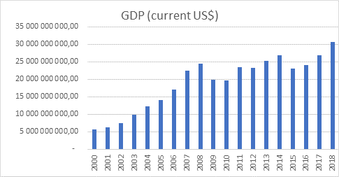
In recent years, Estonia’s GDP has grown steadily by about 9-11%. The exceptions are 2009 and 2015, which can be described as a crisis time for the world’s economy.
Table 1 GDP – Estonia 2000-2018
Regression analysis
We performed a correlation analysis of the relationship between exogenous and endogenous indicators. In this case, endogenous indicator is GDP. Period under review – since 2000 to 2018 year. Currently there is no actual data about 2019 year.
![]() – the endogenous parameter (the GDP), the aim of constructing this model.
– the endogenous parameter (the GDP), the aim of constructing this model.
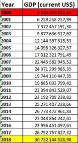
Figure 1 – The data for Y –the GDP in Estonia
Let us consider the major factors (variables), which influence on GDP. There are three exogenous parameters in this model. The GPD is the first one, which are taken with the lag. The lag is equal one year.
![]() – the lagged GDP.
– the lagged GDP.
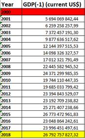
Figure 2 – The data for X1 -lagged GDP
The second parameter is the final consumption expenditure.
![]() – the final consumption expenditure.
– the final consumption expenditure.
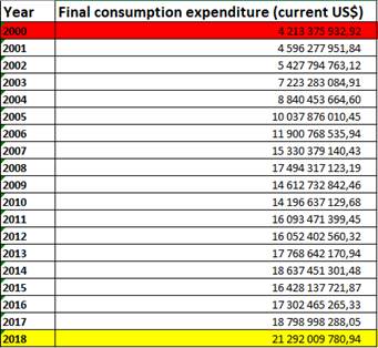
Figure 3 – The data for X2 – final consumption expenditure
The third parameter for our model is the general government final consumption expenditure.
![]() – the general government final consumption expenditure.
– the general government final consumption expenditure.

Figure 4 – The data for X3 – the general government final consumption expenditure
By using the linear regression function in Excel, it is possible to create the linear equation, which calculate coefficient for each exogenous parameter. After that, it can be possible to do conclusion about the relevance of this model, if the model satisfies specific requirements.
Results
Our estimated model is presented below.
![]()
Coefficient of determination (R2adj) equals 0,996. This means that around 99.7 % of the changes of the dependent variable are explained by the changes in the independent variables by the linear regression model.
F-test checks non-randomness of R2 and equality of specification of a linear regression model. As it can be seen, Fcrit equals to 3,197 and F is equal to 1771,05. This means that the coefficient of determination is non-random and quality of specifications on the estimated model is high.
The next rule is the completing T-test. We have to compare T-statistic with P-value. As we can see from the table 1, in absolute value, the T-statistic is higher than the P-value for all coefficients and we may conclude that our coefficients of linear regression are significant.
Table 1 – The data for T-test
|
t-statistic |
P-value |
|
-2,661119263 |
0,019592787 |
|
-1,322755551 |
0,208714235 |
|
13,49369128 |
5,056E-09 |
|
-1,127653658 |
0,279849332 |
After that, check is being performed by three Gauss-Markov conditions. The first condition of Gauss-Markov theorem is that average mean of residuals is equal to zero. In order to check that, the average mean of residuals should be calculated. As it can be seen from the residual table, the average mean of residuals is nearly equal to zero, henсe the first condition of Gauss-Markov theorem is satisfied. This means, that coefficients of the model are unbiased.
In order to check the second Gauss-Markov condition, the Goldfeld-Quandt test can be used. This test checks the homoscedasticity in regression analyses. As it can be seen from the table 2, Fcrit is higher than GQ and 1/GQ.
Table 2 – The Goldfeld-Quandt test calculation
|
GQ |
0,234367 |
|
1/GQ |
4,266815 |
|
FкритGQ |
6,388233 |
In order to check the third Gauss-Markov condition, the Durbin-Watson test should be run. As it can be seen from the results of the test, Durbin-Watson value lies in the yellow zone between dl and du. This means that there is no information about autocorrelation.
Adequacy of the model is checked throughout the construction of the confidence interval. If the real value lies between Y^– and Y^+ the model is adequate. As it can be seen from the table 3, the real value stay between Y^– and Y^+, that’s why the model is adequate.
Table 3 – The Goldfeld-Quandt test calculation
|
Y^2018= |
30 380 736 512,45 |
|
Y^–2018= |
29 577 742 385,46 |
|
Y^+2018= |
31 183 730 639,45 |
|
Y2018= |
30 732 144 528,98 |
Finally, the average approximation variance is equal 1.14%, so this model is relevance for using.
BIBLIOGRAPHY
1. Financial data. https://data.worldbank.org/ [Accessed 24 February 2020].
2. Data and statistic https://countryeconomy.com/ [Accessed 27 February 2020]
3. Трегуб И.В. Прогнозирование экономических показателей на рынке дополнительных услуг сотовой связи. Финансовая акад. при Правительстве Российской Федерации, Каф. Мат. моделирование экономических процессов. Москва, 2009.
4. Трегуб И.В. Математические модели динамики экономических систем: монография – Москва: РУСАЙНС, 2018. – 164 с.
5. Трегуб И.В. Эконометрические исследования. Практические примеры. Econometric studies. Practical examples. – Москва: Лань, 2017. 164 с.
6. Tregub I.V. Econometrics. Model of real system. М.: 2016, 164 p.
7. Трегуб И.В. Эконометрика на английском языке Учебное пособие. М.: 2017.