Introduction
Belgium, a
small and open economy of 11.4 million inhabitants, is located in the heart of
Europe. The economy benefits from a strong communication infrastructure and a
highly qualified workforce.
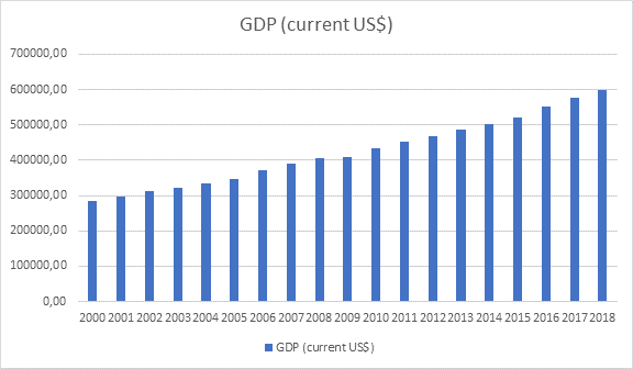
Real GDP
Growth data in Belgium is updated quarterly. Belgium’s GDP expanded 0.4 percent
on quarter in the three months to December 2018, the same as in the previous
period and in line with preliminary estimates. Household consumption (0.5
percent vs 0.7 percent in Q4) and gross fixed capital formation (0.1 percent vs
0.4 percent) slowed while government expenditure rose faster (1.1 percent vs
0.5 percent). Also, foreign demand contributed negatively to growth, as exports
rose 0.6 percent (vs -0.4 percent) and imports increased at a faster 0.9
percent (vs -0.3 percent). Year-on-year, the GDP advanced 1.2 percent, slowing
from a 1.6 percent expansion in the previous period and also matching earlier
estimates. It was the lowest annual GDP growth since Q2 2014. Considering 2018,
the economy advanced 1.4 percent, the least since 2013 and below a 1.5 percent
gain in 2017. So, the data reached an all-time high in 2018 and a record low in
2000 year.
Table
1 GDP – Belgium 2000-2018
Regression
analysis
A correlation
analysis was carried out of the relationship between the endogenous indicator,
which is understood in this case as the GDP and exogenous indicators from 2001
to 2018.
![]() – the endogenous parameter
– the endogenous parameter
(the GDP).
|
Year |
GDP |
|
2000 |
284933,00 |
|
2001 |
296257,00 |
|
2002 |
312900,00 |
|
2003 |
320613,00 |
|
2004 |
333831,00 |
|
2005 |
347658,00 |
|
2006 |
371464,00 |
|
2007 |
390526,00 |
|
2008 |
405729,00 |
|
2009 |
407955,00 |
|
2010 |
434371,00 |
|
2011 |
451933,00 |
|
2012 |
469720,00 |
|
2013 |
487344,00 |
|
2014 |
503620,00 |
|
2015 |
521018,00 |
|
2016 |
550989,00 |
|
2017 |
577535,00 |
|
2018 |
597433,00 |
Figure 1 – The data
for Y –the GDP in Belgium
We study the
main factors (variables) that affect the indicator of GDP. There are two exogenous
parameters in this model. GPD is the first to be taken with a lag. The lag is
one year.
![]() – the lagged GDP.
– the lagged GDP.
|
Year |
GDP |
|
2001 |
284933,00 |
|
2002 |
296257,00 |
|
2003 |
312900,00 |
|
2004 |
320613,00 |
|
2005 |
333831,00 |
|
2006 |
347658,00 |
|
2007 |
371464,00 |
|
2008 |
390526,00 |
|
2009 |
405729,00 |
|
2010 |
407955,00 |
|
2011 |
434371,00 |
|
2012 |
451933,00 |
|
2013 |
469720,00 |
|
2014 |
487344,00 |
|
2015 |
503620,00 |
|
2016 |
521018,00 |
|
2017 |
550989,00 |
|
2018 |
577535,00 |
Figure 2 – The data
for X1 – lagged GDP
The second
parameter for our model is the general government final consumption
expenditure.
![]() – the general government final
– the general government final
consumption expenditure.
|
Year |
General government spending (current US$) |
|
2001 |
12144,00 |
|
2002 |
11990,00 |
|
2003 |
12392,00 |
|
2004 |
12922,00 |
|
2005 |
12992,00 |
|
2006 |
13691,00 |
|
2007 |
17790,00 |
|
2008 |
19174,00 |
|
2009 |
20583,00 |
|
2010 |
21363,00 |
|
2011 |
22598,00 |
|
2012 |
23790,00 |
|
2013 |
24422,00 |
|
2014 |
24719,00 |
|
2015 |
24576,00 |
|
2016 |
25147,00 |
|
2017 |
25818,00 |
|
2018 |
26636,00 |
Figure 3 – The data
for X2 – general government final consumption expenditure
So, let’s
create the linear equation, by using the linear regression function in Excel to
calculate the coefficient for each exogenous parameter. In that case, it is
possible to estimate the relevance of the model.
Results
Our estimated
model is presented below.
![]()
Coefficient of
determination (R2adj) equals 0,995647526340896. This
means that around 99,7 % in changes of dependent variables are explained by
changes in independent variables by linear regression models.
F-test checks
non-randomness of R2 and equality of specification of a linear regression
model. From
calculations it was received, that Fcrit= 3,591530568 and F=1601,28084171368.
So, the
coefficient of determination is non-random and quality of specifications is
high.
Then need to
perform the T-test by comparing the T-statistics with the P-value. As can be
seen from Table 1, in the absolute value, the T-statistic is higher than the
P-value for all the considered coefficients. So, that is why our linear
regression coefficients are significant.
Table
1 – The data for T-test
|
T-statistic |
P-value |
|
-0,709631617 |
0,489583798 |
|
15,78776858 |
2,580811178 |
|
-1,068406623 |
0,303413885 |
Let’s check
the three conditions of the Gauss-Markov.
The first
condition of Gauss-Markov theorem is that average mean of residuals is equal to
zero. In order to check that, the average mean of residuals should be
calculated. As it can be seen from the residual table, the average mean of
residuals is nearly equal to zero, henсe the first condition of Gauss-Markov theorem is satisfied. This means,
that coefficients of the model are unbiased.
The
Goldfeld-Quandt test can be used to check the second Gauss-Markov condition.
This test checks the homoscedasticity in regression analyses. As it can be seen
from the table 2, Fcrit is higher than GQ and 1/GQ.
Table
2 – The Goldfeld-Quandt test calculation
|
GQ |
1,817679422 |
|
1/GQ |
0,550152017 |
|
FcritGQ |
6,094210926 |
In
order to verify the third Gauss-Markov condition, it is necessary to conduct
the Durbin-Watson Test. Based on the test results, it can be noted that the
Darbin-Watson value lies in the yellow zone between dl and du.
Based on it, we can conclude that there is no information about
autocorrelation.
The
adequacy of the model is checked throughout the construction of the confidence
interval. Based on the data from Table 3, we can conclude that the real value
lies between Y^– and Y^+, so, that is why
the model is adequate.
Table
3 – The Goldfeld-Quandt test calculation
|
Y^2018= |
605937,08 |
|
Y^–2018= |
592826,65 |
|
Y^+2018= |
605973,54 |
|
Y2018= |
597433,00 |
Finally,
the average approximation variance is equal 1,42%, mistake of
approximation is more than 25% that means that our model is inaccurate, so this
model is relevance for using.
References
1. Financial data. https://data.worldbank.org/ [Accessed 1 March 2020].
2. Data and statistic https://countryeconomy.com/ [Accessed 3 March 2020]
3. FOD Economic https://economie.fgov.be/ [Accessed 5 March 2020]
4. OECD Economic Surveys https://www.oecd.org/ [Accessed 3 March 2020]
5. Трегуб И.В. Прогнозирование
экономических показателей на рынке дополнительных услуг сотовой связи.
Финансовая акад. при Правительстве Российской Федерации, Каф. Мат. моделирование
экономических процессов. Москва, 2009.
6. Трегуб И.В. Математические модели
динамики экономических систем: монография – Москва: РУСАЙНС, 2018. – 164 с.
7. Трегуб И.В. Эконометрические
исследования. Практические
примеры. Econometric studies. Practical examples. – Москва: Лань, 2017. 164 с.
8. Tregub I.V. Econometrics.
Model of real system. М.: 2016, 164 p.
9. Трегуб И.В. Эконометрика на
английском языке Учебное пособие. М.: 2017